4 minutes
Naive Bayes Classifier in NLP
In this post we explore the Naive Bayes classifer in Natural Language Processing and compute line by line the coefficients from the model from the word counts.
It is a simple model and every single NLP project should start with such a model as a baseline.
Overview
The Naive Bayes Classifier is a simple classification model which assumes that all input features are mutually independant from one another. When used in NLP, it means that each word in the sentence contributes indepedently to the predicted output. To put it simply, it means:
\[P(It\ was\ a\ good\ movie) = P(It) P(was) P(a) P(good) P(movie)\]
As a result, a Naive Bayes classifier becomes a linear model when expressed in log-space:
\[\log P(sentence) = b + \sum w_i \log{p_i}\]
To sumarrize, a Naive Bayes classifier assumes that:
- Each feature is independant, i.e. the probablity of occurrence of each word is independent from one another.
- The order of the words does not matter (this is called the "bag-of-words" assumption).
Math details
The goal of a Naive Bayes classifier is to estimate the probability of an instance \(\mathbf {x}\), represented by a vector \(\mathbf {x} = (x_1,\ldots ,x_n)\), to belong to one of the \(k\) classes of the problem (each class is labelled \(C_k\)). Mathematically, it comes down to computing \( p(C_k\mid \mathbf{x}) \) for an instance \(\mathbf {x}\). Using Bayes' Theorem, this expression becomes:
\[ p(C_k\mid \mathbf{x}) = {\frac {p(C_{k})\ p(\mathbf {x} \mid C_{k})}{p(\mathbf {x} )}} \]
Each element in the formula above are sometimes referred to as:
\[ posterior = \frac{prior \times likelihood}{evidence} \]
Now the Naive Bayes classifer assumes that all the features \((x_1,\ldots ,x_n)\) are mutually independant which, after re-arranging the terms, gives us:
\[ p(C_k\mid \mathbf{x}) = \frac {1}{Z} p(C_k)\prod_{i=1}^{n} p(x_i\mid C_k)\]
Where the evidence \(Z\) is a scaling factor dependent only on \((x_1,\ldots ,x_n)\) and is constant if the values of the feature variables are known.
\[ Z = p(\mathbf {x} )=\sum _{k}p(C_{k})\ p(\mathbf {x} \mid C_{k})\]
In NLP, we assume the underlying word distribution is a multinomial distribution:
\[ p(\mathbf {x} \mid C_{k}) = \frac {(\sum _{i=1}^n x_i)!}{\prod _{i=1}^n x_i!} \prod _{i=1}^n p_{ki}^{x_i} \]
Giving us the final log probabilities:
\[\log p(C_k \mid \mathbf{x} ) \varpropto \log \left(p(C_k) \prod_{i=1}^{n}{p_{ki}}^{x_i}\right) \\ = \log p(C_k) + \sum_{i=1}^n x_{i}\cdot \log p_{ki} \\ = b + \mathbf w_k^{\top}\mathbf{x}\]
Data
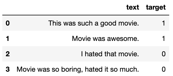
Let's compute the log probabilities manually on a sample dataset and see if our predictions match the ones we obtain when using Python's toolbox. We created this dataset of 4 sentences about movies with 2 positives and 2 negatives:
Then we compute the word count for each sentence and build our count vectorizer:
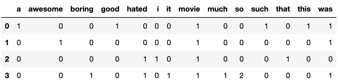
To avoid getting zero counts in some columns which would lead to an error when computing log(0), we add 1 everywhere in the table above. This way of regularizing Naive Bayes is called Laplace smoothing when using a pseudocount other than 1 (parameter alpha in the Python code below). Summing the rows in the table above by target (0 and 1) and then normalizing the result so that the sum of each row is equal to one gives us the following word distributions for each target:
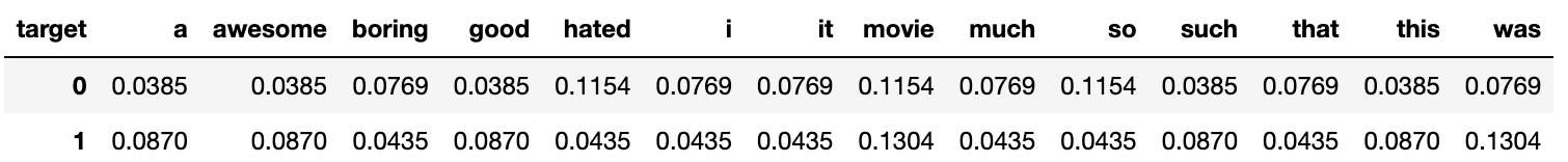
These are word probabilities \(p_{ki}\) for each target, so our log probabilities are:

Using Python's toolbox, we get:
from sklearn.feature_extraction.text import CountVectorizer
from sklearn.naive_bayes import MultinomialNB

# Build sample data
sent1 = "This was such a good movie."
sent2 = "Movie was awesome."
sent3 = "I hated that movie."
sent4 = "Movie was so boring, hated it so much."

sample_data = pd.DataFrame({'text':[sent1, sent2, sent3, sent4], 'target':[1,1,0,0]})

vectorizer = CountVectorizer(token_pattern=r'(?u)\b\w+\b')
X_train = vectorizer.fit_transform(sample_data['text'])
y_train = sample_data['target']

# Multinomial NB
clf = MultinomialNB(alpha=1.0, class_prior=[0.5,0.5]) # alpha is the pseudocount
clf.fit(X_train, y_train)

# Log prob
vocab = vectorizer.get_feature_names()
pd.DataFrame(clf.feature_log_prob_, columns=vocab)
The log probabilities found using Python's toolbox are:

Conclusion
We were able to manually compute the log probabilities for each word in our sample dataset and shed light on how the Naive Bayes classifier makes predictions.